分段线性回归(译文)
By S.F.
本文链接 https://www.kyfws.com/news/segmented-linear-regression/
版权声明 本博客所有文章除特别声明外,均采用 BY-NC-SA 许可协议。转载请注明出处!
- 20 分钟阅读 - 9774 个词 阅读量 0分段线性回归(译文)
原文地址:https://www.codeproject.com/Articles/5282014/Segmented-Linear-Regression
原文作者:Vadim Stadnik
译文由本站翻译
前言
Two algorithms for segmented (piecewise) linear regression 分段(分段)线性回归的两种算法 In this article, we present two algorithms for segmented (piecewise) linear regression: based on sequential search and more efficient but less accurate using simple moving average. 在本文中,我们提出了两种用于分段(逐段)线性回归的算法:基于顺序搜索,使用简单的移动平均值效率更高,但准确性更低.
(Layout) 布局
(Linear Regression) 线性回归
(Linear regression is one of the classical mathematical methods for data analysis, which is thoroughly covered in textbooks and literature. For an introductory explanation, refer to articles in Wikipedia [1]. The large amount of information requires a discussion and a clarification of our approach to this problem.) 线性回归是用于数据分析的经典数学方法之一,其在教科书和文献中都有详细介绍.有关介绍性的解释,请参阅Wikipedia [1]中的文章.大量的信息需要讨论和澄清我们解决此问题的方法. (Linear regression provides an optimal approximation for given data, under the assumption that the data are affected by random statistical noise. Within this model, each value is the sum of a linear approximation in a selected point from the space of independent variables and a deviation caused by noise. In this article, we consider simple linear regression of one independent variable) 假设数据受随机统计噪声影响,则线性回归可为给定数据提供最佳近似值.在此模型中,每个值都是自变量空间中选定点的线性逼近与噪声引起的偏差之和.在本文中,我们考虑了一个自变量的简单线性回归**(*x*) X**(*and one dependent variable*) 和一个因变量**(*y*) ÿ**(*:*) : **(*y*) ÿ**(*i*) 一世(*=*) =**(*a*) 一种**(*+*) +**(*b*) b****(*x*) X**(*i*) 一世(*+*) +****(*i*) 一世 (*where*) 哪里**(*a*) 一种**(*and*) 和**(*b*) b**(*are fitting parameters.*) 是拟合参数.****(*i*) 一世(*represents a random error term of the model. The best fitting is performed using the least-squares method. This variant of linear regression replaces the whole dataset by a single line segment.*) 代表模型的随机误差项.最佳拟合是使用最小二乘法进行的.线性回归的这种变体将整个数据集替换为单个线段. (*As a fundamental mathematical method, linear regression is used in numerous areas of business and science. One the reasons of its popularity is the ability to predict, which is based on the computation of the slope of the approximation line. A large deviation from the line is interpreted as a sign of an important event in a system that changes its behaviour. In data analysis, linear regression provides a clear view of data unaffected by noise. It enables us to create informative diagrams for datasets that may look chaotic at first. This feature is also helpful for data visualization, since it allows us to avoid the art of manual drawing of approximation lines by naked eye. The simplicity and efficiency are important advantages of linear regression over other methods and explain why it is a good choice in practice.*) 作为一种基本的数学方法,线性回归被用于商业和科学的许多领域.其普及的原因之一是预测能力,它是基于近似线斜率的计算得出的.与该线的较大偏差被认为是系统中更改其行为的重要事件的标志.在数据分析中,线性回归提供了不受噪声影响的清晰数据视图.它使我们能够为一开始看起来很混乱的数据集创建信息图.此功能还有助于数据可视化,因为它使我们避免了用肉眼手动绘制近似线的艺术.与其他方法相比,简单性和效率是线性回归的重要优势,并解释了为什么它在实践中是一个不错的选择. (*The limitation of linear regression is that its approximation might become inaccurate when the amount of noise is relatively small (see Figure 1). Because of this, the method does not enable us to reveal inherent features in a given dataset.*) 线性回归的局限性在于,当噪声量相对较小时,其近似值可能会变得不准确(请参见图1).因此,该方法无法使我们揭示给定数据集中的固有特征.
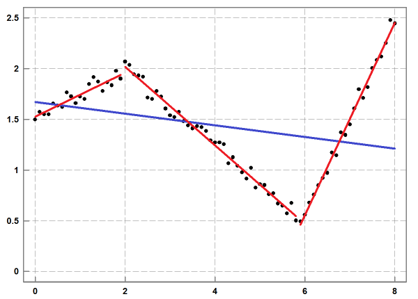
(Figure 1: An example of linear regression (in blue) and segmented linear regression (in red) for a given dataset (in black): the approximation with 3 line segments offers a significantly better accuracy than linear regression.) 图1:给定数据集(黑色)的线性回归(蓝色)和分段线性回归(红色)的示例:3个线段的近似值比线性回归的准确性要好得多.## (Segmented Linear Regression) 分段线性回归 (Segmented linear regression (SLR) addresses this issue by offering piecewise linear approximation of a given dataset [2]. It splits the dataset into a list of subsets with adjacent ranges and then for each range finds linear regression, which normally has much better accuracy than one line regression for the whole dataset. It offers an approximation of the dataset by a sequence of line segments. In this context, segmented linear regression can be viewed as a decomposition of a given large dataset into a relatively small set of simple objects that provide compact but approximate representation of the given dataset within a specified accuracy.) 分段线性回归(SLR)通过提供给定数据集的分段线性逼近来解决此问题[2].它将数据集拆分为具有相邻范围的子集列表,然后针对每个范围找到线性回归,通常,线性回归的准确性要比整个数据集的一线回归好得多.它通过一系列线段来提供数据集的近似值.在这种情况下,分段线性回归可以看作是将给定的大型数据集分解为相对较小的一组简单对象,这些对象在指定的精度内提供了给定数据集的紧凑但近似的表示形式. (Segmented linear regression provides quite robust approximation. This strength comes from the fact that linear regression does not impose constraints on ends of a line segment. For this reason, in segmented linear regression, two consecutive line segments normally do not have a common end point. This property is important for practical applications, since it enables us to analyse discontinuities in temporal data: sharp and sudden changes in the magnitude of a signal, switching between quasi-stable states. This method allows us to understand the dynamics of a system or an effect. For comparison, high degree polynomial regression provides a continuous approximation [3]. Its interpolation and extrapolation suffer from overfitting oscillations [4]. Polynomial regression is not a reliable predictor in applications mentioned earlier.) 分段线性回归提供了非常鲁棒的近似值.这种优势来自以下事实:线性回归不会对线段的末端施加约束.因此,在分段线性回归中,两个连续的线段通常没有公共端点.此属性对实际应用非常重要,因为它使我们能够分析时间数据的不连续性:信号幅度的急剧和突然变化,准稳态之间的切换.这种方法使我们能够了解系统或效果的动态.为了进行比较,高次多项式回归提供了一个连续近似[3].它的内插和外推遭受过拟合振荡[4].在前面提到的应用中,多项式回归并不是可靠的预测指标. (Despite the simple idea, segmented linear regression is not a trivial algorithm when it comes to its implementation. Unlike linear regression, the number of segments in an acceptable approximation is unknown. The specification of the number of segments is not a practical option, since a blind choice produces usually a result that badly represents a given dataset. Similarly, uniform splitting a given dataset into equal-sized subsets is not effective for achieving an optimal approximation result.) 尽管有一个简单的想法,但分段线性回归在实现上并不是一个简单的算法.与线性回归不同,可接受近似中的段数未知.指定段数不是一个可行的选择,因为盲目选择通常会产生不良表示给定数据集的结果.类似地,将给定的数据集均匀拆分为相等大小的子集对于实现最佳逼近结果无效. (Instead of these options, we place the restriction of the allowed deviation and attempt to construct an approximation that guarantees the required accuracy with as few line segments as possible. The line segments detected by the algorithm reveal essential features of a given dataset.) 代替这些选项,我们对允许的偏差进行限制,并尝试构建一个近似值,以尽可能少的线段来保证所需的精度.该算法检测到的线段揭示了给定数据集的基本特征. (The deviation at a specified) 在指定的偏差**(*x*) X**(*value is defined as the absolute difference between original and approximation*) 值定义为原始值与近似值之间的绝对差**(*y*) ÿ**(*values. The accuracy of linear regression in a range and the approximation error are defined as the maximum of all of the values of the deviations in the range. The maximum allowed deviation (tolerance) is an important user interface parameter of the model. It controls the total number and lengths of segments in a computed segmented linear regression. If input value of this parameter is very large, there is no splitting of a given dataset. The result is just one line segment of linear regression. If input value is very small, then the result may have many short segments.*) 价值观.范围内线性回归的准确性和近似误差定义为范围内所有偏差值的最大值.最大允许偏差(公差)是模型的重要用户界面参数.它控制计算的分段线性回归中分段的总数和长度.如果此参数的输入值非常大,则不会拆分给定的数据集.结果只是线性回归的一线段.如果输入值非常小,则结果可能会有很多短段. (*It is interesting to note that within this formulation, the problem of segmented linear regression is similar to the problem of polyline simplification. The solution to this problem provides the algorithm of Ramer, Douglas and Peucker [5]. Nevertheless, there are important reasons why polyline simplification is not the best choice for noisy data. This algorithm gives first priority to data points the most distant from already constructed approximation line segments. In the context of this algorithm, such data points are the most significant. The issue is that in the presence of noise, the significant points normally arise from high frequency fluctuations. The biggest damage is caused by outliers. For this reason, noise can have substantial effect on the accuracy of polyline simplification. In piecewise linear regression, each line segment is balanced against the effect of noise. The short term fluctuations are removed to show significant long term features and trends in original data.*) 有趣的是,在此公式中,分段线性回归的问题类似于折线简化的问题.该问题的解决方案提供了Ramer,Douglas和Peucker的算法[5].但是,有很多重要原因说明为什么折线简化不是嘈杂数据的最佳选择.该算法将与已构造的近似线段最远的数据点赋予最高优先级.在此算法的上下文中,此类数据点最为重要.问题在于,在存在噪声的情况下,有效点通常是由高频波动引起的.最大的损坏是由异常值造成的.因此,噪声会对折线简化的准确性产生重大影响.在分段线性回归中,每个线段都针对噪声效果进行了平衡.去除了短期波动,可以显示原始数据的重要长期特征和趋势.
(Algorithms) 演算法
(Adaptive Subdivision) 自适应细分
(Here, we discuss two algorithms for segmented linear regression. In the attached code, the top level functions of these algorithms are) 在这里,我们讨论了分段线性回归的两种算法.在所附的代码中,这些算法的顶级功能是 SegmentedRegressionThorough() (and) 和 SegmentedRegressionFast() (. Both of them are based on adaptive subdivision, which we borrow from the solution to polyline simplification. Figure 2 shows the top-down dynamics of this method.) .它们都基于自适应细分,我们从解决方案中借用到折线简化.图2显示了此方法的自上而下的动态.
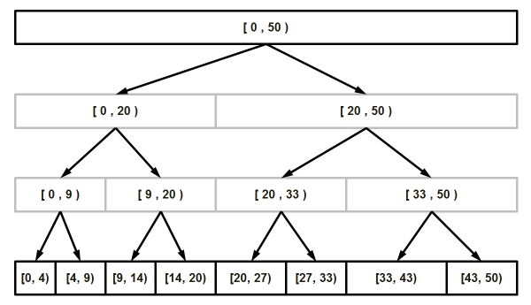
(Figure 2: Illustration of an adaptive recursive subdivision for data stored in an array. The top array represents a given dataset. Each subdivision improves linear regression in two proper arrays at a lower level. The resulting subdivision arrays with required approximation accuracy are located at the deepest level. Note that the arrays are not equal-sized.) 图2:针对数组中存储的数据的自适应递归细分的示意图.最上面的数组代表给定的数据集.每个细分都在较低的水平上改进了两个适当数组中的线性回归.具有所需逼近精度的结果细分数组位于最深的级别.请注意,数组的大小不相等.(The pseudo-code of this subdivision method is given below:) 该细分方法的伪代码如下:
StackRanges     stack_ranges ;
stack_ranges.push( range_top(0, n_values) ) ;

while ( !stack_ranges.empty() )
{
    range_top = stack_ranges.top() ;
    stack_ranges.pop() ;

    if ( CanSplitRange( range_top, idx_split, ... ) )
    {
        stack_ranges.push( range_left (range_top.idx_a, idx_split      ) ) ;
        stack_ranges.push( range_right(idx_split      , range_top.idx_b) ) ;
    }
    else
        ranges_result.push_back( range_top ) ;
}
(The criterion of splitting a range, implemented in both algorithms (see the function) 在两种算法中都实现了划分范围的标准(请参见函数 CanSplitRangeThorough() (and) 和 CanSplitRangeFast() (), is based on the comparison of approximation errors against user provided tolerance. A range is added to the approximation result as soon as the specified accuracy has been achieved for each approximation value in the range. Otherwise, it is split into two new ranges, which are pushed onto stack for subsequent processing.) ),是基于近似误差与用户提供的公差之间的比较.一旦范围内的每个近似值都达到指定的精度,就将范围添加到近似结果中.否则,它将分为两个新范围,将其推入堆栈以进行后续处理.
(These two functions also implement the test for a small indivisible range. It is necessary to avoid confusion that can be caused by the subdivision of a dataset with two data elements only. The current version of the algorithms is not allowed to create a degenerate line segment that corresponds to one datum.) 这两个功能还可以在较小的不可分割范围内执行测试.有必要避免仅将数据集细分为两个数据元素而引起的混淆.当前版本的算法不允许创建与一个基准相对应的简并线段.
(This method of subdivision belongs to the family of divide-and-conquer algorithms. It is fast and guarantees space efficiency of its result. Under the simplifying assumption that the cost of a single split operation is constant, the running time of the recursive subdivision is) 这种细分方法属于分而治之算法家族.它速度快并保证了结果的空间效率.在单个拆分操作的成本恒定的简化假设下,递归细分的运行时间为*(*O*) Ø
*(*(*) (***(*N*) ñ
***(*) in the worst case and*) )在最坏的情况下,*(*O*) Ø
*(*(log*) (日志***(*M*) 中号
***(*) on average, where*) ),平均来说,***(*N*) ñ
***(*is the number of elements in a given dataset and*) 是给定数据集中的元素数,并且***(*M*) 中号
***(*is the number of line segments in a resulting approximation. The cost of a split operation is specific to a particular algorithm. This effect on overall performance is discussed below.*) 是结果近似中的线段数.拆分操作的成本特定于特定算法.下面将讨论对整体性能的影响.
(*The obvious question now is how to find the best split points for the recursive subdivision that we just discussed? It appears that there is more than one method to answer this key question. These methods are responsible for a bit different approximation results and for different performance of SLR algorithms. We start the discussion with the simple method, which is easier to understand than the second more advanced method.*) 现在显而易见的问题是,如何为刚刚讨论的递归细分找到最佳分割点?似乎有多种方法可以回答这个关键问题.这些方法导致略有不同的近似结果和SLR算法的不同性能.我们从简单的方法开始讨论,该方法比第二种更高级的方法更容易理解.
(Sequential Search for the Best Split) 顺序搜索最佳拆分
(The simple method (see function) 简单方法(请参见函数 CanSplitRangeThorough() () represents a sequential search for the best split point in a range of a given dataset. It involves the following computational steps: A currently selected data point provides us with two sub-ranges. For each sub-range, we compute several sums, parameters of linear regression and then the accuracy of the approximation as the maximum of absolute differences between original and approximation) )表示在给定数据集范围内对最佳分割点的顺序搜索.它涉及以下计算步骤:当前选择的数据点为我们提供了两个子范围.对于每个子范围,我们计算一些和,线性回归参数,然后将近似值的精度作为原始值和近似值之间的绝对差的最大值**(*y*) ÿ**(*values. The best split point is defined by the best approximation accuracy for both sub-ranges.*) 价值观.最佳分割点由两个子范围的最佳近似精度定义.
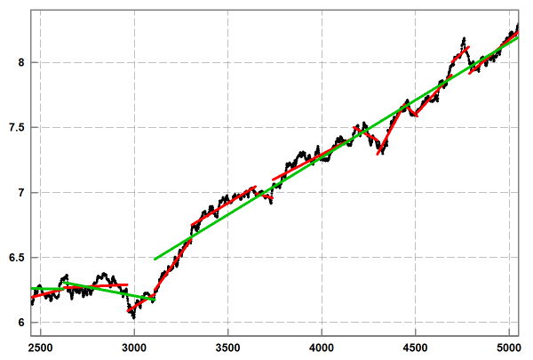
(Figure 3: Segmented linear regression using sequential search for the best split point. The sample noisy data (in black) were obtained from daily stock prices. The lower accuracy approximation (in green) has 3 segments. The higher accuracy approximation (in red) has 13 segments.) 图3:使用顺序搜索的最佳分割点的分段线性回归.样本噪声数据(黑色)是从每日股票价格获得的.较低的精度近似值(绿色)包含3个细分.精度更高的近似值(红色)包含13个细分.(This simple method (see Figure 3) delivers good approximation results in terms of compactness: a small number of line segments for a specified tolerance, but unfortunately it is too slow and not practical for processing large and huge datasets. The weakness of this algorithm is that linear cost of sequential search for the best split in a given range (see function) 这种简单的方法(请参见图3)在紧凑性方面提供了良好的近似结果:对于指定的公差,线段数量很少,但是不幸的是,它太慢了,不适用于处理庞大和庞大的数据集.该算法的弱点是在给定范围内按顺序搜索最佳分割的线性成本(请参见函数 CanSplitRangeThorough() () is multiplied by linear cost of the computation of linear regression in sub-ranges. Thus, the total running time of this algorithm is at least quadratic. In the worst case of linear performance of the recursive subdivision, this algorithm becomes cubic. This speed cannot be improved significantly by using tables of pre-computed sums. The bottleneck is the computation of approximation errors in a range, which takes linear time.) )乘以子范围内线性回归计算的线性费用.因此,该算法的总运行时间至少是二次的.在递归细分的线性性能最坏的情况下,该算法变为三次.使用预先计算的总和表无法显着提高此速度.瓶颈是一定范围内的近似误差的计算,这需要线性时间.
(Search Using Simple Moving Average) 使用简单移动平均线进行搜索
(The efficiency of an algorithm that builds segmented linear regression can be improved if we avoid the costly sequential search on each range discussed in the first algorithm. For this purpose, we need a fast method to detect a subset of data points that are the most suitable to split ranges in a given dataset.) 如果我们避免在第一个算法中讨论的每个范围上进行昂贵的顺序搜索,则可以提高构建分段线性回归的算法的效率.为此,我们需要一种快速的方法来检测最适合在给定数据集中分割范围的数据点子集. (In order to better understand the key idea of the faster algorithm, let us consider perfect input data without noise. Figure 4 shows the computation of simple moving average (SMA) [6] for sample data that have a number of well-defined line segments.) 为了更好地理解更快算法的关键思想,让我们考虑没有噪声的完美输入数据.图4显示了具有多个定义明确的线段的样本数据的简单移动平均(SMA)[6]的计算.
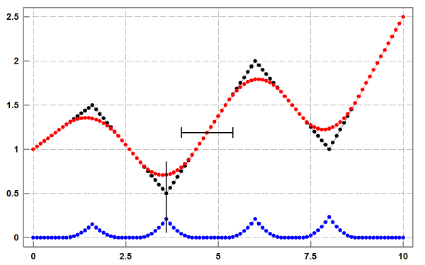
(Figure 4: Simple moving average for sample data not affected by noise: original dataset in black, smoothed data in red, the absolute differences between original and smoothed data in blue. The vertical line illustrates the fact that positions of local maxima in the differences coincide with positions of local maxima and minima in the given data. The horizontal segment denotes smoothing window at a specific data point.) 图4:不受噪声影响的样本数据的简单移动平均值:黑色的原始数据集,红色的平滑数据,蓝色的原始数据和平滑数据之间的绝对差.垂直线示出了在给定数据中差异处的局部最大值的位置与局部最大值和最小值的位置一致的事实.水平段表示特定数据点处的平滑窗口.(The important fact is that when SMA window is inside a range of original data with linear dependence) 重要的事实是,当SMA窗位于一系列线性相关的原始数据中时**(*y*) ÿ**(*(*) (**(*x*) X**(*) each derived*) )每个派生**(*y*) ÿ**(*value is equal to a matching original*) 值等于匹配的原件**(*y*) ÿ**(*value. In other words, the operation of smoothing based on SMA does not affect data points in ranges of linear dependence*) 值.换句话说,基于SMA的平滑操作不会影响线性相关范围内的数据点**(*y*) ÿ**(*(*) (**(*x*) X**(*) of original data. The deviations between original and derived*) )的原始数据.原始和派生之间的偏差**(*y*) ÿ**(*values become noticeable and increasing when smoothing window is moving into a range that covers more than one line segment. In a more general context, the smoothed curve is sensitive to all types of smooth and sharp non-linearities in original dataset, including “corners” and “jumps”. The greater non-linearity, the greater the effect of the smoothing operation.*) 当平滑窗口移至覆盖多个线段的范围时,这些值将变得明显并增加.在更一般的情况下,平滑曲线对原始数据集中的所有类型的平滑和锐利非线性敏感,包括"角"和"跳".非线性越大,平滑操作的效果越好.
(*This feature of SMA suggests the following method to find ranges of linear dependence*) SMA的这一特征建议采用以下方法来找到线性相关性的范围**(*y*) ÿ**(*(*) (**(*x*) X**(*) for the computation of local linear regression and break points between them. If we compute the array of absolute differences between original and smoothed values, then the required ranges of linear dependence in original data correspond to small (ideally zero) values of differences in this array. The break points between these approximation ranges are defined by local maxima in the array of differences.*) )计算局部线性回归和它们之间的折点.如果我们计算原始值和平滑值之间的绝对差数组,则原始数据中所需的线性相关性范围对应于此数组中的较小(理想值为零)的差值.这些近似范围之间的断点由差异数组中的局部最大值定义.
(*In the algorithm implemented in the attached code (see function*) 在所附代码中实现的算法中(请参见函数 SegmentedRegressionFast() (*), we detect all local maxima in the array of absolute differences between original and smoothed data. The order of splitting approximation ranges (in function*) ),我们会检测原始数据和平滑数据之间的绝对差数组中的所有局部最大值.分割近似范围的顺序(在函数中 CanSplitRangeFast() (*) is determined by the magnitude of local maxima. For each new range of subdivision, we compute parameters and approximation error of linear regression. This processing stops as soon as a required accuracy has been achieved. It means that not all of the local maxima are normally used to build the approximation result.*) )由局部最大值的大小决定.对于每个新的细分范围,我们都计算线性回归的参数和近似误差.一旦达到所需的精度,该处理就会停止.这意味着通常不是所有局部最大值都可用于构建近似结果.
(*When it comes to real life data affected by noise (see Figure 5), smoothing not only helps us to detect line segments in given data, but also allows us to measure the amount of noise in the data. The current version of this algorithm uses symmetric window. The length of the window provides control of the accuracy of linear approximation. In order to obtain smoothed data, we apply one smoothing operation to the whole input dataset. There is no need later to use smoothing in approximation ranges created by subdivision. This approach helps us to avoid issues associated with boundary conditions of SMA.*) 对于受噪声影响的现实生活数据(请参见图5),平滑处理不仅可以帮助我们检测给定数据中的线段,还可以测量数据中的噪声量.该算法的当前版本使用对称窗口.窗口的长度可控制线性逼近的精度.为了获得平滑的数据,我们对整个输入数据集应用了一种平滑操作.以后无需在细分创建的近似范围内使用平滑.这种方法有助于我们避免与SMA边界条件相关的问题.
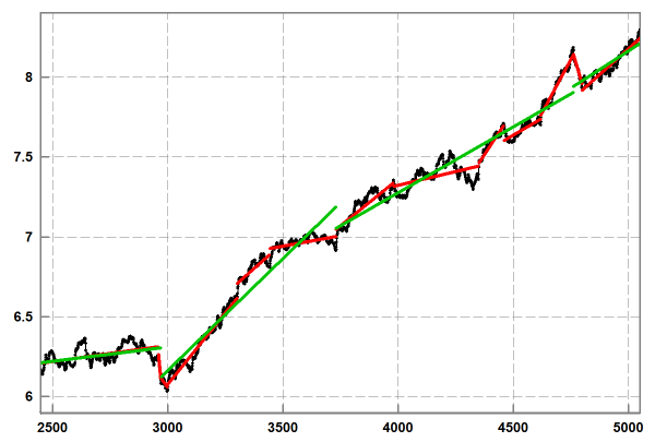
(Figure 5: Segmented linear regression using simple moving average for the same data as in Figure 3. The lower accuracy approximation (in green) has 4 segments. The higher accuracy approximation (in red) has 13 segments.) 图5:对于图3中的相同数据,使用简单移动平均值进行分段线性回归.较低的精度近似值(绿色)有4个细分.精度更高的近似值(红色)包含13个细分.(It should be clear from this discussion that the choice of a smoothing method is important for this variant of piecewise linear regression. SMA is a low pass filter. Thus, it looks like other types of low pass filters are suitable for smoothing operation too. This is not impossible in theory, but it is unlikely that this is a good idea in practice. Compared to other types of low pass filters, SMA is one of the simplest and efficient. Its properties have been intensively studied. In particular, a well-known issue of SMA is that it can invert high frequency oscillations. For the algorithm discussed here, this will lead to a bit less accurate locating local maxima. This issue can be easily addressed with iterative SMA, which is known as Kolmogov-Zurbenko filter [7]. In addition, iterative SMA gives more control over the removal of high frequency fluctuations. Not only smoothing window length but also the number of iterations is available to reduce the amount of noise in derived data and to achieve the best possible approximation. Importantly, this iterative filter also preserves line segments of given data.) 从该讨论中应该清楚,平滑方法的选择对于分段线性回归的这种变型很重要. SMA是低通滤波器.因此,看起来其他类型的低通滤波器也适用于平滑操作.从理论上讲这不是不可能的,但实际上这不是一个好主意.与其他类型的低通滤波器相比,SMA是最简单有效的方法之一.已经对其性质进行了深入研究.尤其是,SMA的一个众所周知的问题是它可以反转高频振荡.对于此处讨论的算法,这将导致定位局部最大值的精度降低.这个问题可以通过迭代SMA轻松解决,它被称为Kolmogov-Zurbenko滤波器[7].此外,迭代SMA可以更好地控制高频波动的消除.不仅可以平滑窗口长度,而且可以使用迭代次数来减少派生数据中的噪声量并实现最佳近似.重要的是,此迭代过滤器还保留给定数据的线段.
(In terms of performance, the second SLR algorithm (function) 在性能方面,第二个SLR算法(功能 SegmentedRegressionFast() () has the important advantage over the first algorithm (function) )比第一种算法(函数 SegmentedRegressionThorough() (). The costs of major algorithmic steps are not multiplied but added. The search for potential split points using local maxima in absolute differences between original and smoothed data is quite fast and is completed before the recursive subdivision. This search involves the computation of SMA, an array of differences and an array of local maxima. Since each of these computations takes linear time, this stage of algorithm also completes in linear time. The subsequent recursive subdivision operates on the given split points and only needs to compute parameters of local linear regression, which takes linear time. Thus, the average cost of this SLR algorithm is) ).主要算法步骤的成本不会增加,而会增加.使用原始最大值和平滑数据之间的绝对差异中的局部最大值来搜索潜在的分割点的速度非常快,并且在递归细分之前已完成.该搜索涉及SMA,差值数组和局部最大值数组的计算.由于这些计算中的每一个都需要线性时间,因此该算法阶段也将在线性时间中完成.随后的递归细分在给定的分割点上进行运算,只需要计算局部线性回归的参数,这需要线性时间.因此,此SLR算法的平均成本为*(*O*) Ø
*(*(*) (***(*N*) ñ
***(*log*) 日志***(*M*) 中号
***(and the worst case cost is quadratic, where*),最坏的情况是二次费用,其中***(*N*) ñ
***(*is the number of elements in a given dataset and*) 是给定数据集中的元素数,并且***(*M*) 中号
***(*is the number of line segments in resulting approximation. This performance is much better than that of the first algorithm. This is why the algorithm based on smoothing is the preferable choice for the analysis of large datasets.*) 是得到的近似值中线段的数量.这种性能比第一种算法要好得多.这就是为什么基于平滑的算法是分析大型数据集的首选方法的原因.
(*The price of the improved performance is that the second algorithm may not find precise positions of split points that guarantee the highest accuracy of linear regression. This is often acceptable in real life applications, since the exact position of a local maximum in noisy data is a bit vague concept. This situation is similar to the analysis of smoothed data. An approximation is normally acceptable as soon as its smoothed curve is meaningful in the application context. A failure to find segmented linear regression when user tolerance is strict is not necessarily a bad feature of this algorithm. If there are two line segments in input data, the algorithm is not expect to detect ten approximation line segments. As an additional measure, the precision of finding best split points can be improved by using narrow sequential search in areas of local maxima only.*) 改进性能的代价是第二种算法可能无法找到保证线性回归的最高准确性的分割点的精确位置.这在现实生活的应用程序中通常是可以接受的,因为在噪声数据中局部最大值的确切位置有点模糊的概念.这种情况类似于平滑数据的分析.通常,只要在应用程序上下文中有意义的平滑曲线有意义,就可以接受这种近似.当用户公差严格时,找不到分段线性回归不一定是该算法的一个坏功能.如果输入数据中有两个线段,则该算法不会检测到十个近似线段.作为一项附加措施,可以通过仅在局部最大值区域中使用狭窄的顺序搜索来提高找到最佳分割点的精度.
(*For large and huge datasets, the performance and accuracy can be controlled by combining two algorithms: First, we run fast algorithm based on SMA smoothing to detect significant split points. This result is used for initial partition of a given dataset to build the first order approximation. Then, we continue subdivision of the ranges of the first approximation with sequential search for split points that has better accuracy.*) 对于庞大和庞大的数据集,可以通过组合两种算法来控制性能和准确性:首先,我们运行基于SMA平滑的快速算法来检测重要的分割点.该结果用于给定数据集的初始分区,以建立一阶近似值.然后,我们继续对第一近似值的范围进行细分,并依次搜索具有更好准确性的分割点.
(Concluding Remarks) 结束语
(It is interesting to note the implementation of both algorithms requires a small amount of code. The comments in the attached code are focused on the appropriate technical details. In this section, we discuss the other important aspects of the code and algorithms.) 有趣的是,两种算法的实现都需要少量代码.随附代码中的注释集中在适当的技术细节上.在本节中,我们将讨论代码和算法的其他重要方面.
(In order to focus on the main ideas of the algorithms, their implementation prioritizes readability of the code. For the same reason, we do not use the methods that address issues of numerical errors in computations, which involve floating-point numbers. This approach makes the code more portable to other languages. In this context, we note that class) 为了专注于算法的主要思想,它们的实现优先考虑代码的可读性.出于同样的原因,我们没有使用解决涉及浮点数的计算中的数字错误问题的方法.这种方法使代码更易于移植到其他语言.在这种情况下,我们注意到 std::vector<T> (represents a dynamic array. Also, the implementation is not optimized for the best performance. In particular, it does not use tables of pre-computed sums or advanced data structures.) 代表动态数组.此外,该实现未针对最佳性能进行优化.特别是,它不使用预计算总和表或高级数据结构.
(As discussed before, the attached code does not support a user interface parameter for the minimal length of a range (the limit for indivisible range). The implementation of these general purpose algorithms applies the fundamental limit of 2 points for a line segment. Because of this, segmented linear regression can have many small line segments, which correspond to data subsets with small number of elements produced by subdivision process. This effect is usually caused by high frequency noise when user specified accuracy of approximation is too strict. Such a result most likely is not useful in practice. If this is the case, then it makes sense to introduce a larger limit for indivisible range to detect the failure at early stages of processing.) 如前所述,附件代码不支持范围最小长度(不可分割范围的极限)的用户界面参数.这些通用算法的实现对线段应用2个点的基本限制.因此,分段线性回归可以具有许多小线段,这些线段对应于细分过程产生的具有少量元素的数据子集.当用户指定的近似精度太严格时,这种影响通常是由高频噪声引起的.这样的结果很可能在实践中没有用.如果是这种情况,则有必要对不可分割范围引入较大的限制,以在处理的早期阶段检测故障.
(The algorithms discussed here assume that input data are equally spaced. It is possible to use these algorithms in special cases when deviations from this requirement are relatively small. However, in the general case, it is necessary to properly prepare input data. The issue of outliers is beyond the scope of this article, although it is very important in practice. The current implementation assumes that all input values are significant and none of them can be removed.) 此处讨论的算法假定输入数据的间距相等.在与该要求的偏差相对较小的特殊情况下,可以使用这些算法.但是,在一般情况下,必须正确准备输入数据.异常值的问题超出了本文的范围,尽管在实践中非常重要.当前实现假定所有输入值都是有效的,并且不能删除任何输入值.
(Segmented linear regression becomes ineffective when it contains a large number of small segments (loss of compactness) or its representation of data does not achieve a specified accuracy. Another complication is that segmented linear regression allows for more than one acceptable result. This fact makes its interpretation not as trivial as that of linear regression.) 当分段线性回归包含大量小段(紧凑性损失)或者其数据表示未达到指定的准确性时,它将变得无效.另一个复杂因素是分段线性回归可以得到多个可接受的结果.这一事实使其解释不像线性回归那样简单.
(In practical applications, the naïve questions “what is noise?” and “what is signal?” quite often are hard to answer. However, without the knowledge of characteristics of noise, we cannot make reliable conclusions and meaningful predictions. The major challenge is to develop an adequate mathematical model for the data analysis. The models that work well are thoroughly tested against real life datasets.) 在实际应用中,天真的问题是"什么是噪音?“和"信号是什么?“很多时候很难回答.但是,如果不了解噪声的特征,就无法做出可靠的结论和有意义的预测.主要挑战是为数据分析开发适当的数学模型.效果良好的模型已针对实际数据集进行了全面测试.
(References) 参考文献
-
(https://en.wikipedia.org/wiki/Linear_regression) https://zh.wikipedia.org/wiki/线性回归
-
(https://en.wikipedia.org/wiki/Polynomial_regression) https://zh.wikipedia.org/wiki/多项式回归
-
(https://en.wikipedia.org/wiki/Overfitting) https://zh.wikipedia.org/wiki/过度拟合
-
(https://en.wikipedia.org/wiki/Moving_average) https://zh.wikipedia.org/wiki/移动平均
(History) 历史
- (7) 7(th) 日(October, 2020: Initial version) 2020年10月:初始版本
许可
本文以及所有相关的源代码和文件均已获得The Code Project Open License (CPOL)的许可。
C++ Intermediate 新闻 翻译